Comprehensive genome analysis and variant detection at scale using DRAGEN

Over the last decade, the advent of genomic sequencing as a common methodology in genomics, genetics and medical applications has enabled multiple discoveries and insights for diseases, population diversity, evolutionary mechanisms and personalized medicine strategies^1,2,3,4. This was made possible in large part due to improvements in next-generation sequencing (that is, Illumina) in terms of costs, high data quality and scalability¹. Highly accurate methods for the detection of single-nucleotide variations (SNVs) and smaller (<50 bp) insertions or deletions (indels) have been at the forefront of variant detection and interpretation. Despite the amount of attention that SNVs have garnered, they are not the only variant type that differentiates two genomes^5,6. Recently, an increasing number of studies incorporate structural variation (SV)^7,8,9 into their analysis. SVs are often defined to be 50 bp or larger and lead to deletions, insertions, amplifications or rearrangements of a genome⁷. Copy number variation (CNV) is another genomic variation that arises from deletions (loss of copies) or duplications (gain of copies) of a specific DNA segment⁷. Another understudied variant type is short tandem repeat (STR) expansions that are mainly defined by their low sequence entropy/complexity^10,11. These types of variants have been associated with many diseases, diversity and evolutionary patterns. Their detection and interpretation remain challenging, but multiple specialized methods have been proposed^5,7. Although all of these variant types are present across genomes, many studies often focus on only SNVs or subsets of variant types independently due to the challenges of joint detection and accurate reporting of the variant classes. Additional challenges arise from highly diverse and repetitive regions of the genome that further complicate analysis^6,12. Although these variant types likely interact together, these relations are lost when analyzed independently. Thus, more comprehensive approaches that can scale are required.

One proposed way to unify variant discovery is via specialized sequencing technologies, that is, long reads, that have been reported to improve certain aspects such as SV detection (for example, Oxford Nanopore Technologies (ONT) or PacBio)^5,7. These technologies have matured substantially over the past few years and are becoming more commonly available⁵. However, long-read technologies are still often limited by their cost, data quality and scalability and more often by their sample requirements in terms of quantity and quality⁵. This often hinders their application across larger populations or even legacy samples. Interestingly, what these sequencing technologies have demonstrated is that the alleles that are identifiable using their long reads are also often present and identifiable in short reads¹³. This has been most successfully shown in SV genotyping using graph genomes^13,14. Recent improvements, including graph genome approaches, have been shown to improve SV genotyping and the mapping of short reads¹⁵. Nonetheless, these methods often pose challenges to apply them at scale and thus have often been applied to only reidentify certain alleles (that is, genotyping)¹⁶making their utility very limited¹⁵. Single improvements need to act together to fully detangle the complex genomic landscape of an individual, even more so on a population scale.

The current trend is often to not only identify and interpret variants in only the coding regions of the genome but also investigate the impact of variants across the entire genome using whole-genome sequencing (WGS), which further adds to the complexity of the challenges due to repetitiveness (for example, segmental duplications), complex polymorphisms and the lack of variant annotations^6,17. The central question to address these challenges is what is needed to improve the interpretation of all variant types to identify novel candidate disease alleles or genes. To tackle this, the typical approach is to increase the number of samples that are analyzed to obtain robust population allele estimations. This motivated multiple large-scale studies (for example, Centers for Common Disease Genomics¹⁸Trans-Omics for Precision Medicine (TOPMed)¹⁹All of US and UK Biobank (UKBB)) focusing on Illumina sequencing, which substantiates the role of short reads as the workhorse of genomics and genetics. It also requires a scalable and unified software framework to comprehensively identify all variant types (SNVs, indels, SVs, CNVs and repeat expansions), which has not been realized⁶. A framework capable of this would not only scale the identification of the variation landscape from a single genome to millions of genomes but also enable us to obtain key insights into multiple adult diseases that are currently poorly understood due in part to focus on SNVs^20,21.

Here, we present dynamic read analysis for genomics (DRAGEN) and its optimization in SNV and indel calling and its ability to detect the entire landscape of variations (CNVs, SVs, repeat expansions and specialized methodologies for certain regions such as HLA, SMN, GET, LPA and other genes with clinical significance (see Table 1)). These developments bring together advancements in genomic algorithm development to address long-standing issues of scalability, accuracy and comprehensiveness of variant detection across all sizes and types of alleles and thus fully resolve individual genomes cost effectively at scale. The accuracy of DRAGEN is boosted by a multigenome mapper implementation that scales and enables the detection of variant types beyond just SNVs. In this study, we introduce and benchmark DRAGEN’s 14 subcomponents (SNVs, SVs, STRs, CNVs, nine targeted callers, including four new callers, and the gVCF genotyper) and illustrate their ability to scale across large cohorts by analyzing the 1000 Genome Project (1kGP)²². We reveal new insights into the diversity of the genome across populations with a special focus on medically relevant genes to demonstrate the genomic and medical utility of DRAGEN. We introduce methods to compare and merge the variants produced to further emphasize DRAGEN’s ability to analyze multiple variant classes together. This includes SNV and indel merging strategies to scale and produce fully genotyped population variant call format (VCF) files. Similarly, we provide solutions to combine STRs, SVs and CNVs into one population VCF file. Both methods allow the handling of all variant types together and promote the assessment of mid- to large variants for cohort studies. We demonstrate this across 3,202 whole-genome samples from the 1kGP cohort. This study showcases how DRAGEN can address some of the challenges and limitations of clinical genomics with discovery of accurate and potentially novel variants linked to disease in studies of both common and rare conditions.

Algorithms for comprehensive genomics at scale and accuracy

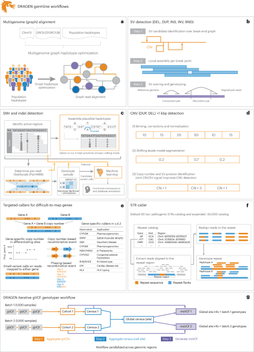
In this paper, we present a framework (DRAGEN v.4.2.4) to identify all types of genomic variations at scale and cost. Figure 1 provides a brief overview of DRAGEN’s main components. First, each sample is mapped to a pangenome reference, consisting of a reference and several assemblies, for example, GRCh38 in addition to 64 haplotypes (32 samples) together with reference corrections previously reported²³ to overcome errors on the human genome. The pangenome reference includes variants from multiple genome assemblies to better represent sequence diversity between individuals throughout the human population. Briefly, the seed-based mapping considers both primary (for example, GRCh38) and secondary contigs (phased haplotypes from various populations) throughout the pangenome. The alignment is controlled over established relationships of primary and secondary contigs and is adjusted accordingly for mapping quality and scoring (see Supplementary Information for details). DRAGEN’s mapping process for a 35× WGS paired-end dataset requires approximately 8 min of computation time using an onsite DRAGEN server (Supplementary Table 1 provides details of the time taken in each step for both an Amazon Web Services (AWS) F1 instance and an onsite Phase4 server). The pangenome reference can be updated with advancements (for example, T2T-CHM13 or HPRC pangenome assemblies) and can enable a more precise and comprehensive alignment of the short reads. These improved alignments are leveraged for variant calling.

To identify SNVs and indels (<50 bp), DRAGEN assembles regions with variants using a de Bruijn graph, which is then input to a hidden Markov model with previously estimated noise and error levels per sample. The output is a (g)VCF file. The SNV caller has key innovations to deal with noise or sequencing errors, including (1) sample-specific PCR noise estimation, (2) correlated pileup errors estimation, (3) consideration of overlapping candidate events and (4) local assembly failures and incomplete haplotype candidates. After the initial variant calling, a machine learning framework rescores calls to further reduce false-positive small variants (both SNVs and indels) and recover wrongly discarded false negatives (see Fig. 1 and Supplementary Information for details).

Simultaneously, DRAGEN identifies SVs (≥50 bp genomic alterations) and copy number events (≥1 kbp genomic alterations) using two methods (see Fig. 1 and Supplementary Information for details). For SV calling, DRAGEN extends Manta²⁴ by introducing the following key concepts that substantially improve SV calling: (1) a new mobile element insertion detector for large insertion calling, (2) optimization of proper pair parameters for large deletion calling, (3) improved assembled contig alignment for large insertion discovery, (4) refinements to the assembly step, (5) refinements in the read likelihood calculations step, (6) improved handling of overlapping mates, (7) improved handling of clipped bases and (8) filtering and precision improvements (see Fig. 1 and Supplementary Information for details). For CNV calling, DRAGEN targets 1 kbp and larger variants that cause an amplification or deletion of genomic segments. This CNV caller uses a modified shifting levels model, which identifies the most likely state of input intervals through the Viterbi algorithm (see Fig. 1 and Supplementary Information for details). The CNV caller was also designed to take into consideration the discordant and split-read signals from the SV calling to detect events down to 1 kbp. Furthermore, DRAGEN identifies STR mutations and analyzes known pathogenic genomic regions using a method primarily based on ExpansionHunter²⁵.

Some important genes are challenging to genotype due to their high sequence similarity to pseudogenes, repetitive regions and polymorphic nature. To overcome these challenges, DRAGEN integrates nine targeted callers for accurate genotyping of clinically relevant genes (CYP2B6, CYP2D6, CYP21A2, GET, HBA, LPA, RH, SMN and HLA), of which six of the callers are described here^26,27,28,29. In general, DRAGEN uses common SNVs in the population to distinguish gene targets from their paralogous copies to provide copy number estimations for each haplotype. Furthermore, DRAGEN identifies reads that do not follow the general phasing patterns and reports the recombination events that lead to these reads per sample (see Supplementary Information for details on each caller). The CYP2D6 and CYP2B6 genes are important for pharmacogenomics and encode an enzyme that is responsible for metabolizing most commonly used drugs³⁰. The recombination of gene and pseudogene can lead to deletions of part of each copy, generating gene–pseudogene fusions. The variants across CYP21A2 can lead to congenital adrenal hyperplasia³¹. GET is an important target gene due to variants that increase the risk for Parkinson’s and Gaucher’s disease and Lewy body dementia^32,33. The gene resides in a segmental duplication of 10 kbp with a pseudogene GBAP1. The high sequence homology in GET/GBAP1 drives homologous recombination and can result in pathogenic gene conversions or CNVs. HLA encodes proteins crucial for immune regulation and response and holds immense importance in research related to autoimmune diseases, organ transplantation and cancer vaccines and immunotherapy^34,35. DRAGEN includes a specialized caller to identify HLA class I (HLA-A, HLA-B and HLA-C) and class II (HLA-DQA1, HLA-DQB1 and HLA-DRB1) alleles. Mutations in the HBA genes (HBA1 and HBA2) cause α-thalassemia, an inherited blood disorder characterized by lowered levels of α-globin, a fundamental building block of hemoglobin³⁶. Recurrent homologous recombination can result in 3.8 kbp deletions that create a hybrid copy of HBA1 and HBA24.2 kbp deletions that delete regions that include the HBA2 gene or complete deletion of both. Small pathogenic variants can also be detected within HBA. The LPA gene includes a 5.5 kbp region (KIV-2) whose copy numbers (between 5 and 50+) are inversely related to cardiovascular risk³⁷. DRAGEN can report phased copy numbers for this region²⁹. For RHD/RHCE (RH blood type), copy number predictions can be used to assess the risk of Rh allosensitization³⁸. Another integrated caller identifies CNVs across SMN1 and SMN2which can indicate spinal muscular atrophy²⁷.

The genome-wide simultaneous assessment for SNVs, indels, STRs, SVs and CNVs together with reporting the results from these specialized callers takes approximately 30 min of computation time with an onsite DRAGEN server for a 35× WGS sample. This results in a gVCF file for SNVs and indels, a VCF file for each STR, CNV and SV calls and tabular formats for the specialized gene callers (Fig. 1).

Thus, the DRAGEN pipeline is able to capture the entire range from single variants to larger variations across the entire genome at scale and reports them in standardized VCF files. The algorithms are described in detail in Supplementary Information. This pipeline aims to produce a comprehensive and accurate set of genomic variations across the human genome at scale.

Resolving the complete variant spectrum at scale and accuracy

We applied DRAGEN to the HG002 sample, for which multiple benchmarks are available^{16,39,40,41,42}. We identified variants using DRAGEN across a 35× coverage HG002 Illumina NovaSeq 6000 2 × 151 bp paired-end read dataset (Methods). Figure 2a shows the distribution of all small and large variants across the HG002 sample and highlights the ability of DRAGEN to capture the entire variant spectrum. This resulted in ~4.92 million small variant calls that includes 3,956,307 SNVs with a transition-to-transversion ratio of 1.98 and an SNV heterozygous-to-homozygous (HET/HOM) ratio of 1.56. A total of 960,908 indels were discovered with an insertions-to-deletion ratio of 1.00 and HET/HOM ratio of 1.865. For SVs, 13,886 variants (≥50 bp) were identified with 5,901 deletions, 7,174 insertions, 42 duplications, 153 inversions and 616 translocations. Additionally, 1,156 CNVs were identified ranging from 1 kbp to 445 kbp with a deletion-to-duplication ratio of 4.25. DRAGEN detected STR expansions or contractions in 31,370 polymorphic loci out of the 50,069 in the STR catalog (homozygous reference 0/0: 37.33%, heterozygous 0/1: 27.36%, homozygous alternate 1/1: 17.8% and heterozygous genotype composed of two different alternate (ALT) alleles 1/2: 17.5%). Relative to GRCh38, 46.66% (14,636) of HG002 STRs have at least one more copy and 53.34% (16,734) have at least one less copy, thus highlighting all the variant complexities that a single genome represents.

Using these results, all the variants were evaluated against the Genome in a Bottle (GIAB) benchmarks and compared to other short-read-based callers (Methods). For SNVs and indels, benchmark v.4.2.1 was used on GRCh38 (ref. ⁴⁰), but for the SV benchmark (v.0.6) (ref. ³⁹), DRAGEN was run on a GRCh37 version of the pangenome reference. Later, the benchmark was expanded across the challenging medically relevant gene (CMRG) catalog⁴¹ (see Methods for details). Over all benchmarks, DRAGEN demonstrated higher accuracy and impressive speed up of the analysis from raw reads to finalized variant calls within 30 min total, which is better than any other existing workflow.

We first focused on SNV and indel calling for HG002 and compared its performance to other short-read-based methods⁴³ (GATK⁴⁴ and DeepVariant⁴⁵ with BWA⁴⁶). We further benchmarked the recent pangenome approach Giraffe¹⁵. Figure 2b shows the F-measures across SNV and indel results (see Supplementary Table 2 for details). Overall, we observed a clear advantage of SNV identification accuracy relative to other methods. For the overall genome-wide small variant calls, DRAGEN achieved an F-measure of 99.86%, yielding a total of 11,163 errors (2,553 false positives and 8,610 false negatives). Compared to DRAGEN, we observed 2.49 times more errors for DeepVariant + BWA calls (F-measure: 99.64%, 3,695 false positives and 24,090 false negatives), 1.79 times more errors for DeepVariant + Giraffe calls (F-measure: 99.74%, 4,980 false positives and 15,021 false negatives) and 6.07 times more errors for GATK + BWA calls (F-measure: 99.13%, 38,622 false positives and 29,163 false negatives) with the same Illumina sample. This is in part due to the methodologies implemented in the SNV calling and in the subsequent machine learning filtering (see Supplementary Information). We observed improvements for SNV and indel (2–50 bp) variant types. DRAGEN achieved a higher F-measure of 99.86% (SNV) and 99.80% (indel) than GATK + BWA, DeepVariant + BWA and DeepVariant + Giraffe (Supplementary Table 2). Thus, clearly, DRAGEN showed an improved performance on SNVs and indels across the entire spectrum, improving the characterization across samples at scale.

We next assessed the performance of variant calling in the CMRG catalog. This GIAB benchmark spans 273 medically relevant genes that are highly repetitive and diverse and were therefore excluded from the genome-wide benchmark¹². Many of these medically relevant genes overlap segmental duplications and other challenging properties. There is interest to see if short-read sequencing can be used effectively for detecting variants in these repetitive regions. Moreover, several of these medically relevant genes (for example, KCNE1, CBS, CRYAA, KCNJ18, MAP2K3, KMT2C) are wrongly represented in the GRCh38 reference due to false duplication and collapsed sequence errors²³. Corrections to these errors have been incorporated into DRAGEN variant calling. Figure 2c shows the results of the individual SNV callers with respect to F-measure (see Supplementary Table 2 for details on the evaluations). For both SNV and indel calls, DRAGEN (F-measure: 98.64%) was better than GATK (95.84%), DeepVariant + BWA (97.32%) and DeepVariant + Giraffe (98.10%). These improvements are present in both SNVs and indels (Supplementary Table 2), thus outperforming the other methods with 13,931 variants across the genome and 509 variants in CMRG regions, which are only identifiable by DRAGEN. We further investigated if this performance differed between exonic and intronic regions. For the exonic regions, DRAGEN achieved an F-measure of 99.78%. For intronic and intergenic regions, the achieved F-measures were 99.87% and 99.85%, respectively. Similarly, variant calling performance was evaluated on exonic and intronic regions using the GIAB CMRG benchmark set. DRAGEN achieved F-measures of 98.97% and 98.66% on exonic and intronic regions, respectively.

In addition to the clear improvements of DRAGEN for SNVs (Fig. 2b,c), DRAGEN’s performance across SVs (>50 bp) was also improved. The DRAGEN results were compared to SV calls reported by Manta²⁴Delly⁴⁷ and Lumpy⁴⁸ (Fig. 2d,e and Methods). For insertions, which are often the hardest for SV callers⁷WEAR achieved an F-measure of 76.90%, which more than doubled the performance of Manta (34.90%) and Delly (4.70%; Lumpy did not report any insertions). This is due to multiple algorithmic innovations in DRAGEN (Supplementary Information). Similarly, DRAGEN achieved a better F-measure (82.60%) for deletions (50+ bp) than Manta (70.80%), Delly (68.30%) and Lumpy (66.80%). Supplementary Table 3 contains details across the SV types. DRAGEN’s performance was also compared for SV detection on CMRG regions. DRAGEN again outperformed the other variant callers with F-measures of 63.50% and 68.00% for insertion (Fig. 2d) and deletion (Fig. 2e) types, respectively. This showcases the ability of short reads to detect SVs with high accuracy even in repetitive regions.

DRAGEN also reports CNVs, which include larger deletions and duplications. Here, CNVs are adjusted for the called SV to improve breakpoint accuracy where possible (see Supplementary Information). The performance was compared to that of the CNVnator⁴⁹ copy number discovery tool and benchmarked using the>1 kbp deletion SV records from the GIAB SV benchmark set (Fig. 2f). For CNVs with lengths in the range of 1–5 kbp and 5–10 kbp, DRAGEN performed substantially better, with F-measures of 92.60% (versus 39.20% for CNVnator) and 96.60% (versus 61.80% for CNVnator), respectively. For CNVs with lengths in the range of 10–20 kbp, 20–50 kbp and>50 kbp, similar performances by DRAGEN (F-measures of 94.10%, 95.20% and 100.00%, respectively) and CNVnator (97.60%, 94.90% and 99.00%, respectively) were observed. Supplementary Table 4 contains all the benchmarking results.

Similar to SVs, STRs are often challenging to resolve due to their repetitiveness and complexity⁵⁰. The accuracy of STR detection by DRAGEN was evaluated using the GIAB tandem repeat benchmark dataset (GIABTR) v.1.0 (ref. ⁵⁰) and Truvari⁵¹. For the STR caller, we assessed two catalogs that are available in DRAGEN that differ in the number of STR loci analyzed. The first catalog consists of 50,069 regions where the F-measure (19.68%) was largely driven by the small size of the catalog compared to the 1.7 million regions represented in GIABTR, which impacts recall. Nevertheless, the precision was high at 95.47%. When using the larger STR catalogs available in DRAGEN, which include 174,300 regions, the F-measure improved to 55.13% with the same precision. To provide context to these results, we benchmarked another short-read caller, GangSTR⁵²and compared its performance to DRAGEN’s performance (Fig. 2g and Supplementary Table 5). Because GangSTR is optimized for a different set of 832,380 regions, we evaluated performance on the intersection of both methods’ analyzed regions against GIABTR (~174,000; Methods). When restricting the benchmark to the intersection between the two catalogs, DRAGEN achieved a better F-measure of 96.72% (versus 69.86% by GangSTR). When we extended the benchmark to cover all DRAGEN catalog regions, DRAGEN’s F-measures for ~50,000 and ~174,000 catalogs were 94.56% and 94.47%, respectively, whereas GangSTR achieved an F-measure of 62.55% (shown as recall and F-measure in Fig. 2g). Given that this benchmark includes mostly small variants within tandem repeat loci, both the DRAGEN small variant caller and DRAGEN STRs were evaluated against the benchmark. The DRAGEN small variant caller achieved an F-measure of 93.7% when compared to the entire GIABTR benchmark and an F-measure of 87.9% when restricting the comparison to indels larger than 5 bp, indicating that DRAGEN can accurately detect SNVs and small indels in tandem repeat regions and that such events represent the majority of tandem repeat variants in any given genome. The true-positive and true-negative overlaps between the STR caller and small variant caller were 93.67% and 99.49%, respectively, for ~174,000 catalog regions (Supplementary Fig. 1).

Last, the performances of all targeted callers were evaluated using orthogonal datasets (Table 1), and DRAGEN calls showed high concordance for all results. The callsets for HG002 were analyzed for each targeted caller. There are two pharmacogenomics-related methods that assess CYP2D6 and CYP2B6 alleles. For HG002, the caller reported *1/*U1;*2/*5 star alleles for CYP2B6 and *2/*4 for CYP2D6. The *1 and *U1 alleles in the first genotype represent the reference allele and specific variant in the gene that has reduced enzyme activity, respectively. Similarly, the second genotype, *2/*5, indicates that the HG002 sample may carry two different variants of the CYP2B6 gene, which reduces enzymatic activity. The CYP2D6 caller for HG002 generated *2/*4 star alleles, which indicates that the sample carries two haplotype variants that are also associated with reduction in the enzyme activity of the gene. The methods for HBA1/HBA2 (α-thalassemia) reported no detected target variants. The CYP2D6 and CYP2B6 callers had 99.3% and 92.1% concordance of star allele calls, respectively, against orthogonal calls in a cohort of samples characterized by Get-RM⁵³. The CYPB26 caller results were also concordant against the long-read-based (PacBio) calls (Table 1). DRAGEN HLA typing on sample HG002 revealed HLA-A*01:01, HLA-A*26:01, SONG-B*35:0, SONG-B*38:0, HLA-C*04:01 and HLA-C*12:03 class I alleles and HLA-DQA1*01:05, HLA-DQA1*03:01, HLA-DQB1*03:02, HLA-DQB1*05:01, HLA-DRB1*10:01 and HLA-DRB1*04:03 class II alleles. The class I genotyping results were perfectly concordant with other callers, such as HLA-LA⁵⁴HISAT-genotype⁵⁵T1K⁵⁶ and HLA*ASM⁵⁷. For HLA class II, the results from DRAGEN were also highly concordant with those from other tools (HLA*ASM gets one allele wrong on HLA-DQA1) except for the HLA-DRB1 allele (improvement pending in DRAGEN). We also compared the Optitype results from 164 samples from the 1kGP samples, and the overall accuracy of DRAGEN (98.27%) was similar to that of Optitype (98.43%; Supplementary Table 6).

For the SMN caller, HG002 had ‘negative’ affected status and carrier status, 0 copy numbers of SMN2Δ7–8 (deletion of exons 7 and 8) and 3.77 estimated total copy numbers, indicating four haplotypes across the two genes. Benchmarking of the SMN caller showed that 99.8% of SMN1 and 99.7% of SMN2 copy number calls agreed with orthogonal methods (MLPA/droplet digital PCR).

The GET caller assesses GET and GBAP1 recombinations and variants that can be important for neurological diseases²⁸ and reports whether the sample is biallelic or not for pathogenic variants, the total copy number, and carrier status. For the HG002 sample, DRAGEN reported four total copy numbers and ‘False’ for both ‘is_bi-allelic’ and ‘is_carrier’ fields. Benchmarking showed that GET calls were 100% concordant with targeted long-read-based methods (ONT) across 42 samples with diverse variant types.

The LPA caller assesses LPA copy number status, which provides important information on cardiovascular disease risk²⁹. Interestingly this method provides phasing information for approximately 50% of the samples. HG002 has 39 KIV-2 LPA repeats with allele-specific (alleles 1 and 2) copy numbers of 25 and 14, respectively. These methods are highly specialized for their individual targeted regions of the genome and report important allelic information rather than variants (for example, a single SNV). The benchmark results showed 98.2% and 99.7% correlation between DRAGEN-estimated KIV-2 total copy numbers and allele-specific copy numbers respectively, against KIV-2 copy numbers extracted from Bionano optical mapping across 154 samples. Supplementary Table 6 contains the descriptions of the callers and results for the HG002 sample.

Because STR, SV and CNV calls each cover a broad range of variant lengths, it is possible for a single variant to be present in more than one result. Therefore, we developed a procedure to combine DRAGEN STR, SV and CNV calls together to form a comprehensive deduplicated large variant VCF file using Truvari⁵¹. The merge procedure analyzed a total of 55,414 variants for HG002 and identified 993 redundant variant representations. To establish the accuracy of the merging, the variants that are labeled SV were extracted from the merged file, and benchmarking was performed using the GIAB SV (v0.6) callset. The benchmarking results of the original SV calls were compared with the benchmarking results after merging and were found to be nearly identical, with only 36 variant representations altered enough to change their benchmarking status (Supplementary Fig. 2).

Benchmarking the DRAGEN pipeline shows that it produces accurate results that improve variant performance across all variant types and lengths. The pipeline generates a fully comprehensive representation of a human genome, including all variant types at scale and cost.

Improving variant identification across the human population

With the performance of DRAGEN on HG002 characterized, we next applied the pipeline to other standard GIAB reference samples to assess the accuracy and comprehensiveness of DRAGEN across multiple ancestries. These samples include the HG001 (NA12878) sample, the parent samples of AshkenazimTrio (HG003 and HG004) and the ChineseTrio samples (HG005, HG006 and HG007). Figure 3a shows an overview of the results across variant types and size regiments. An average of 4,894,415 small variants were detected per sample with an average of 3,952,885 SNVs and 941,530 indels per sample. A balance (ratio: 0.999) between small insertions an d deletions was observed. The mean SNV transition-to-transversion ratio was observed to be 1.98, and the total HET/HOM ratio was observed to be 1.49. For SVs (≥50 bp), the mean SV count per sample was 14,734, with a range between 14,093 and 15,224 per individual. Across samples, insertions (mean: 48.78%) were the most frequently occurring SV type, followed by deletions (mean: 39.10%), translocations (mean: 5.20%), inversions (mean: 1.37%) and tandem duplications (mean: 0.36%; Supplementary Table 7). This follows the expected distributions of insertions being the most frequent variant type, which is typically not observed by other Illumina-based methods⁷. DRAGEN calls other variants, such as CNVs, STRs and variants for some complex and medically relevant genes. On average, 632 CNVs per sample (range between 583 and 718) were detected, with lengths between 1 kbp and 500 kbp (Supplementary Table 7). The STRs were detected across 50,069 loci, including 62 known pathogenic loci for each sample. Across the samples, an average of 13,690 heterozygous and 8,901 homozygous STR variant calls were identified.

DRAGEN performance was then evaluated against the GIAB v.4.2.1 benchmarks for samples HG001–HG007 for SNVs and indels⁴⁰. The recall for genome-wide calls was in the range of 99.76% and 99.87% with precision between 99.90% and 99.93% (Supplementary Table 7). For SNVs and indels, the mean F-measures were 99.80% and 99.87%, respectively (Fig. 3b). This shows a remarkably high consistency across all samples in the performance to identify SNVs and indels. DRAGEN SNV call performance was then compared to that of GATK and DeepVariant calls with BWA and Giraffe¹⁵ mapper using the GIAB benchmark for all samples (Fig. 3c,d and Methods). Across all callers and samples, the F-measure was shown to be below that of DRAGEN (GATK: 99.10% to 99.28%; DeepVariant + BWA: 99.61% to 99.71%). The higher F-measure is largely attributed to improved detection of SNVs and indels (Supplementary Table 7). Benchmarking across all seven samples (HG001–HG007) allows further assessment of the ability of DRAGEN to use a pangenome reference. Figure 3c shows the accuracy of DRAGEN compared to the accuracy obtained by aligning on the HPRC reference pangenome with Giraffe¹⁵ and variant calling with DeepVariant⁴⁵the BWA⁵⁸ with DeepVariant pipeline and the GATK pipeline. Compared to GATK + BWA, DRAGEN showed an average error reduction of 82.88% on combined SNVs and indels, with an average reduction of 83.95% on SNVs and 76.19% on indels. Compared to DeepVariant + BWA, DRAGEN showed an average error reduction of 60.07% on combined SNVs and indels, with an average reduction of 62.40% and 46.46% on SNVs and indels, respectively, confirming the trend observed in the previously reported precisionFDA V2 samples⁵⁹. Compared to Giraffe + DeepVariant, DRAGEN reported an average error reduction of 44.33% on combined SNVs and indels, with an average of 45.57% on SNVs and 39.19% on indels. Furthermore, we evaluated the effect of the pangenome reference on DRAGEN variant calling performance. On average, the pangenome reference reduced the error by 54.20% for samples HG001–HG007 for SNVs and indels, with an average reduction of 57.74% on SNVs and 29.52% on indels (Supplementary Table 7).

Because these samples are trios (Ashkenazim (HG002, HG003 and HG004) and Chinese (HG005, HG006 and HG007)), the variant calling was further validated based on Mendelian inconsistencies. The percentages of genotypes at which a trio had ‘no missingness’ and ‘no Mendelian error’ for DRAGEN were found to be 97.70% and 96.58% for the AshkenazimTrio and ChineseTrio samples, respectively, when genome-wide analysis was performed. For the DeepVariant (with the BWA-MEM mapper) callsets, the rates were 97.34% and 96.95% for HG002–HG004 and HG005–HG007, respectively. Of note is that DeepVariant joint callsets had 23,838 and 37,003 more variants with missing genotypes than the DRAGEN joint callset for the Ashkenazim and Chinese trios, respectively. When considering GIAB high-confidence regions that encompass 88.43% of the genome and excluding certain complex segmental duplications and centromere regions, the ‘no missingness and no error’ for DRAGEN improved slightly with 99.85% and 99.67% for the respective trios. The DeepVariant results also showed similar performance with 99.85% and 99.75% for these two trios, respectively. Furthermore, DeepVariant joint calls had 8,065 and 20,833 more variants than DRAGEN for the respective trios. The observed de novo variant rate for both trios on the DRAGEN callset was 0.05% (Methods and Supplementary Table 7).

Comprehensive variant detection at population scale using DRAGEN

We next applied DRAGEN to discover variants in the well-studied high-coverage 1kGP^22,23 samples and analyze the catalog of genomic variation at population and cohort levels. The 1kGP samples consist of a total of 3,202 samples from 26 different populations of five different ancestry (that is, superpopulation) groups: African (AFR), European (EUR), South Asian (SAS), East Asian (EAS) and American (AMR). This collection of samples contains 1,598 (49.91%) men and 1,604 (50.09%) women. The AFR samples have the highest number of samples (n = 893, 27.89%), followed by the EUR (n = 633, 21.64%), EAS (n = 601, 18.77%), SAS (n = 585, 18.27%) and AMR (n = 490, 15.30%) samples. Recently, the low-coverage (7.4×) WGS datasets²² of 2,504 samples in 1kGP have been expanded to 3,202 high-coverage (35×) datasets⁶⁰. We analyzed the 1kGP samples with DRAGEN to compare with the recently published SNV callset⁶⁰ with GATK and SV callset with a combination of three tools (GATK-SV⁶¹svtools⁶² and Absinthe⁶³). Analysis with DRAGEN showed an improved performance of variant callings in terms of novel small variants (that is, SNVs and indels) and SVs⁶⁰.

For this analysis, it is important to have accurate single-sample calling methodologies and methods that combine VCF files from multiple individuals. It is also important to be able to annotate the variants rapidly and accurately. To accomplish this, a new gVCF merge method for SNVs and indels was implemented (see Supplementary Information). We used Truvari to combine STRs, SVs and CNVs together. This resulted in two-population merged VCF files, one for small variants (that is, SNVs and indels) and one for larger variant classes.

For small variants (<50 bp), the DRAGEN Iterative gVCF Genotyper can efficiently aggregate hundreds of thousands to millions of gVCFs to perform joint calling and genotyping. This generates a fully genotyped population VCF file, which is needed for any genome-wide association studies, rare variant studies, phasing and imputation and ancestry studies. The output population VCF file also contains cohort-level variant statistics (including allele frequency, sample genotype rate and coverage rate) and quality control metrics (such as Hardy–Weinberg test P value and inbreeding coefficient) that can be used for downstream variant filtering (see Supplementary Information for details). Before aggregation, variants with DRAGEN machine learning quality scores below a threshold of QUAL = 3 were filtered. The joint callset had an average per-sample SNV recall of 99.92%, precision of 99.78% and F1-measure of 99.85% and indel recall of 99.84%, precision of 99.71% and F1-measure of 99.77%, as evaluated based on GIAB samples. The aggregation of over 3,202 samples took approximately 2 h on an Illumina Phase4 server with a concurrency of 200 jobs.

For STRs, SVs and CNVs, the variants were first combined on a per-individual level to remove redundant variant representations across types using Truvari⁵¹. Truvari compares the alleles and sizes together with the location and the type of variant event (for example, deletions versus insertions). Supplementary Fig. 2 shows this across sample HG002 with remarkably similar performance values on SVs only and merged STR, SV and CNV results. After this first step per individual, individuals at the population level were merged.

Population-level SNV and indel identification

We applied DRAGEN across 3,202 high-coverage (35×) 1kGP samples to perform comprehensive variant calls (SNVs, indels, SVs, STRs and CNVs) and demonstrate scalability. The variants were analyzed, and the results were compared to published results⁶⁰. At the cohort level, DRAGEN identified 116,346,215 SNVs and 24,979,420 indels. The principal component analysis (PCA) plot (Fig. 4a) for the small variants at the cohort level showed distinct clusters for different populations, which demonstrates shared genetic ancestry among samples. The distribution of SNVs and indels at the population level showed that the AFR superpopulation has the highest number of SNVs and indels (Fig. 4b,c) due to the higher diversity of the AFR group, but this is also likely impacted by the high number of AFR samples in the cohort (Supplementary Table 8). The average SNVs per sample ranged from 3,930,793 (EUR) to 4,771,879 (AFR) and followed expected diversity⁶⁰. The number of small insertions (<50 bp) for the EAS group (521,068) was the lowest and was the highest for the AFR group (626,296). This was interestingly inverted when small deletions (<50 bp) were assessed. The highest proportion of singletons (28.7%) was observed in the AFR population, which also follows previous findings. However, the EAS population had the highest mean number of singletons (that is, ratio of total singletons for a population and the number of samples) compared to other populations.

The allele frequency-based analysis on 2,504 unrelated samples showed that DRAGEN generated 55,327,091 (52.05%) singleton, 38,210,741 (35.68%) rare (allele frequency ≤ 1%) and 13,163,982 (12.27%) common (allele frequency > 1%) SNVs. Compared to a previous GATK callset on these samples, it generated 2.15% more singletons, 0.98% fewer rare and 1.63% fewer common SNVs (Fig. 4d,e). For indels, DRAGEN generated 7,140,867 singleton, 8,237,880 rare and 4,229,692 common indels, whereas the GATK callset had 56.18% fewer singleton (3,129,240), 30.48% fewer rare (5,727,021) and 4.88% fewer common indel variants (4,023,422). Using the Illumina Connected Annotations (ICA)⁶⁴ pipeline (see Supplementary Information), the variants detected by both the DRAGEN and GATK callsets were compared to known SNVs (dbSNP build 155) to determine which variants were previously observed (that is, known) or previously unobserved, to our knowledge (that is, novel). The majority of SNVs (88.98%) from DRAGEN were known, and 72.74% of indels were known variants. The singleton rate of known variants was 52.05% of SNVs and 36.42% of indels (Supplementary Table 9).

Although most SNVs and indels were rare, the novel rate of indels with a functional impact was between 9% and 15% across samples, whereas the SNV novel rate was between 1% and 3%. Specifically, among SNVs with functional impact, DRAGEN called 706,355 missense SNVs (33.13% rare and 1.75% novel), 438,735 synonymous SNVs (36.59% rare and 1.18% novel) and 195,345 SNVs with other higher functional impact, including stop/start–gain/loss and splice mutations (33.35% rare and 3.17% novel). For indels with a functional impact, DRAGEN called 24,047 frameshift indels (27.40% rare and 12.60% novel), 22,079 in-frame indels (38.78% rare and 8.28% novel) and 30,978 indels with other higher functional impact, including stop/start–gain/loss and splice mutations (39.04% rare and 10.07% novel; Fig. 4f,g and Supplementary Table 10). We compared the functional annotations of the DRAGEN callset with those of the GATK callset (Fig. 4f,g). In the intronic, intergenic and regulatory regions, more SNVs and indels were called by DRAGEN than by GATK. In these annotation categories, the percentage of rare and novel variants (in particular indels) was higher in DRAGEN than in GATK. In annotation categories with low to high functional impact, DRAGEN called fewer missense, synonymous and functional impact SNVs. The percentage of rare SNVs was higher and the percentage of novel SNVs was lower in the DRAGEN callset. Frameshift indels and indels with a functional impact were higher in DRAGEN and were found to have a lower allele frequency than GATK. The novel rate was similar between the two callsets but varied between categories due to overall lower numbers of indels in these categories.

The larger number of singletons and novel small variants (<50 bp; SNVs and indels) could highlight DRAGEN’s increased ability to assess repetitive regions of the genome, which is enabled due to the multigenome mapping implementation (see Supplementary Information). To answer this, we first focused on the CMRG regions that are important for clinical analysis. We analyzed the variants identified by DRAGEN in 389 challenging gene regions and compared them to the previous GATK-based results. DRAGEN identified 1,125,183 (0.80% of total) variants in those regions. This is similar to the GATK results of 1,146,580. Next, we investigated if DRAGEN accurately captures the variants in 12 medically important genes that are underrepresented on GRCh38 (ref. ²³). These 12 genes comprise 9 that are incorrectly duplicated and 3 that are incorrectly collapsed (for example, two instead of three copies). These regions include the genes KMT2C, H19, MAP2K3, KCNJ18, KCNE1, CBS, U2AF1, CRYAA, TRAPPC10, DNMT3L, DGCR6 and PRODH. For the nine genes that are incorrectly duplicated, DRAGEN was able to circumvent this bias and reported 30,306 variants. This is in stark contrast to the GATK callset, which reports almost 19.98% fewer (24,249) variants. As an example, for CBSrelated to cystathionine β-synthase deficiency⁶⁵only 221 variants were reported across 1kGP in a previous study⁶⁰. DRAGEN reported 1,196 variants in the callset due to the use of the multigenome mapping. For the H19 gene, which is related to skeletal muscle disease⁶⁶DRAGEN found 335 variants; however, GATK found no variants. For genes that were impacted due to collapsed errors, we expected an inflated number of variants due to multiple haplotypes collapsing on top of each other²³. For MAP2K3which is related to skin and liver diseases⁶⁷and KCNJ18which is related to other rare diseases⁶⁸GATK discovered 487 more variants than DRAGEN, which are likely false positives²³ (Supplementary Table 11).

Unification of large alleles across 3,202 individuals

We next investigated the larger variants identified by DRAGEN encompassing STRs (50,069 regions), SVs and CNVs. As described above, we merged all large variant types across the samples into one population VCF file. We identified 409,033 STRs (243,083 expansions (that is, the reference had fewer repeat units) and 165,950 contractions (that is, the reference had more repeat units)), 1,013,541 SVs (with 200,713 deletions, 450,581 insertions and 28,574 tandem duplications and 333,673 other types of SV) and 9,216 CNVs (5,322 deletions and 3,894 duplications) across the entire 1kGP dataset (Supplementary Table 12). We first performed a PCA to investigate if these calls followed the expected population structure. Figure 5a shows the PCA colored by superpopulation. Overall, we observed a clear separation following the population structure in PC1 and PC2. The large variant PCA had a highly similar structure as that observed in the small variant PCA. The stratification is likely also driven by the higher variant numbers that we observed across the AFR population than observed across the other ancestries, which is also similar to the structure that we observed in the small variant PCA. Figure 5b,c shows the distribution of insertions and deletions per population. Across all SV types, we observed the expected distributions of variant counts with a slight increase of insertions over deletions. Although it remains challenging to identify insertions from short reads, we observed the relatively high numbers of DRAGEN insertions obtained following the general population structure. Figure 5d shows the average number of SVs per individual for each population. Interestingly, although we observe increases in insertions and deletions in the AFR population compared to other populations, the same was not observed for duplications or inversions.

We next investigated how many of these variants have been identified previously^19,60. For this task, we used ICA to annotate variant intersections to 1kGP, gnomAD and TOPMed. Across all variants, we observed 616,371 known variants and 1,035,684 novel variants. Supplementary Table 13 contains the distribution based on allele frequency. To cross check the consistency of the dataset, we correlated the allele frequency of the callsets for the overlapping variant calls. We observed a positive correlation (Pearson correlation coefficient = 0.999, P = 0.0) between allele frequency and the count of variants from the 1kGP database. We next checked for the overlap of variants with exonic, intronic and intergenic regions. A total of 31,223 SVs (7,058 deletions, 9,932 insertions and 14,233 other types of SV) overlapped exonic regions, 558,706 overlapped intronic regions (254,483 insertions, 108,601 deletions and 195,622 other types of SV) and 423,612 overlapped intergenic regions (186,166 insertions, 85,054 deletions and 152,392 other types of SV).

We obtained further insight into SV diversity along medically important genes. As the 1kGP samples represent healthy individuals, their SVs could be used as controls in studies aiming to identify potentially pathogenic variants. We compared DRAGEN SVs to results that were recently published⁶⁰ from a joint calling ensemble approach (GATK-SV⁶¹svtools⁶² and Absinthe⁶³). Across the 5,030 CMRG regions, DRAGEN identified 338,108 variants (268,850 SVs, 66,371 STRs and 2,887 CNVs). The SV callset that was published in recent studies reported only 27,166 SVs, with 8,093 insertions, 13,506 deletions and 5,567 other types of SV. DRAGEN discovered 40,810 more deletions and 90,693 more insertions. Within these medically relevant genes, there are 12 genes that are often negatively impacted by reference bias²³. As mentioned before, some genes suffer from wrongly collapsed copies, which leads to an increased number of variants²³. On the other hand, there are several genes that have been wrongly reported multiple times across the genome, which often leads to missing variant calls due to their repetitiveness²³. For the duplicated and collapsed regions, a total of 101 and 188 large variants were identified by DRAGEN, and the majority of them are SVs (98.02% and 96.86%). By contrast, the previous study only reported 36 SVs in collapsed and 18 SVs in duplicated regions across the entire 1kGP sample. At the cohort level, on average, each individual had 11 variants that were identified in the erroneous regions. For the AFR population, the average number of variants was 13, and for other populations it was between 9 and 10 variants per sample. The distributions of the total number of variants by DRAGEN at the duplicated erroneous regions are higher than the numbers reported in the previous studies, and the numbers are lower in the collapsed regions. This shows the improvement of variant calling by DRAGEN that incorporates the corrected regions during variant calls (Fig. 5e and Supplementary Table 14). A lower number of variants is expected in the collapsed erroneous regions if the corrected reference is used as these erroneous regions in the original GRCh38 reference with more than one copy are collapsed into one.

Insights across complex medically relevant genes for 1kGP

Last, we investigated results from the DRAGEN specialized gene callers (for example, CYPB26, CYPD26 (ref. ²⁶), GET²⁸, HLA and SMN1 and SMN2 (ref. ²⁷)) to obtain deeper insights into potential preconditions across the 1kGP dataset. Furthermore, this dataset can be leveraged as population controls for these important but complex genes.

For the CYP2B6 caller, 2,017 samples had genotypes containing two haplotype-specific star alleles (filter status PASS), 1,174 samples had more than one possible genotype, and 11 samples (10 AFR and 1 EUR) had no calls reported. The metabolizer status reported in these calls showed that among samples with PASS filter, 1,189 were normal metabolizers, 381 were poor metabolizers, 154 were rapid metabolizers, 7 were ultrarapid metabolizers, 224 were intermediate metabolizers, 57 had indeterminate status, and 1,190 had none status. 858 samples had the *1/*1 genotype, and among the samples with multiple genotypes, 945 of them had genotype ‘*1/*6;*4/*9’.

For CYP2D6 calls across all samples, only two samples (one EUR and one SAS) had more than one possible genotype. There were 12 with no calls (2 AFR, 1 SAS, 6 EAS and 3 AMR), and the remaining 3,188 samples had one genotype with two haplotype-specific star alleles. The metabolizer status showed that 1,556 samples had normal status, 781 had intermediate status, 66 had poor status, 107 had ultrarapid status, 149 had indeterminate status, and 543 had none status.

The results of the CYP21A2 caller showed that the total copy numbers were in the range between two and eight, with 58.87% of samples having a copy number of four. For copy numbers greater than or equal to five, there were 687 (21.46%) samples, and 55.31% of samples were from the Asian population (EAS or SAS). It was also reported that 24 samples had copy numbers of less than or equal to three, and a deletion recombinant variant was detected in CYP21A2.

For the GET²⁸ caller that detects both recombinant-like and non-recombinant-like variants in the GET gene, DRAGEN reported no samples with any presence of a recombinant-like variant on each chromosome (homozygous variant or compound heterozygous). However, it reported 13 samples (3 AFR, 5 EUR, 1 AMR, 1 SAS and 3 EAS) with the presence of a recombinant-like variant on only one chromosome. The reported total copy number values showed that the majority of samples (95.47%) had aggregate copy numbers of four across genes and pseudogenes. Only 16 samples had an aggregate copy number of three, and the remaining 129 samples (101 AFR, 1 EUR, 6 AMR, 6 EAS and 15 SAS) had aggregate copy numbers in the range between five and ten. GBA reported only one sample (of EAS) that had one deletion breakpoint in the GET gene, which indicates whether the sample has one of the recombinant-like deletion variants.

For the SMN caller, DRAGEN reported spinal muscular atrophy affected status as ‘false’ for all samples and spinal muscular atrophy carrier status as ‘true’ for 49 (1.53%) samples (3 AFR, 19 EUR, 12 AMR, 7 EAS and 8 SAS). This is in the range of rates of carriers, which is between 2.50% and 1.67% across the population⁶⁹. The copy number of SMN1 was reported to be two for the majority of samples (2,428), and it was not reported for 19 samples (none for SMN1_CN). For SMN2395 samples had zero copies, 1,275 had a copy number of one, 1,427 had a copy number of two, 86 had three or four copies and 19 had no reported copy number.

The DRAGON HLA caller reports HLA typing results of six class I alleles (that is, HLA-A1, HLA-A2, HLA-B1, HLA-B2, HLA-C1 and HLA-C2) and reported 60 distinct alleles for HLA-A170 for HLA-A2121 for HLA-B1132 for HLA-B243 for HLA-C1 and 57 for HLA-C2. For the HLA-A1 type, HLA-A*02:02 was reported to be the allele with the highest allele frequency of 15.8%, followed by HLA-A*11:01 with 11.62%, and the remaining alleles were within 0.03% and 10.06%. For HLA-A2the allele HLA-A*02:01 was reported to have the highest allele frequency of 13.34%, and all others were within 0.03% and 9.90%. For HLA-B1the allele SONG-B*07:0 had the highest allele frequency of 6.71%, and the remaining alleles were between 0.03% and 5.78%. For HLA-B2the SONG-B*35:0 allele had the highest allele frequency of 6.62%, and the remaining alleles were between 0.03% and 5.68%. For HLA-C1the highest allele frequency of 17.36% was reported for the allele HLA-C*04:01and the remaining alleles were in the range between 0.03% and 13.46%. Last, for HLA-C2again the allele HLA-C*04:01 was reported to have the highest allele frequency of 12.05%, and the other alleles were within 0.03% and 8.81%. The allele frequency distribution of HLA type 1 classes among all 1kGP populations is shown in Fig. 5f. Supplementary Table 15 provides details for HLA type counts.

The LPA caller reported the total copy numbers for all 3,202 samples and allele-specific copy numbers for 1,507 (47.06%) samples. The highest and lowest estimated total copy numbers were 80.76 and 11.62, respectively, and both were SAS samples. For allele-specific copy numbers, the highest and lowest were found to be 60.25 and 1.99, respectively, for the first haplotype and 47.90 and 1.99, respectively, for the second haplotype. The distribution of total copy number counts showed that 80% of the samples were between 30 and 50.

The RH caller results showed that the total copy numbers in the RHD and RHCE regions were in the range between two and five. The majority (63.65%) of the samples had total copy numbers of four, and 29.76% samples had total copy numbers of three. For RHD gene regions, 63.49% of samples had a copy number of two, and 29.92% of samples had a copy number of one. It was also observed that 200 samples had copy numbers of zero, and only 13 samples had a copy number of four. For RHCE regions, 99.63% of samples had a copy number of two, only five samples had a copy number of one, and seven samples had a copy number of three.

Thus, here, we have demonstrated the accuracy and scalability of the DRAGEN framework across all variant types. We have demonstrated this across all different variant classes across a wide spectrum of human populations and with a focus on genome-wide and medically relevant genes. This revealed many variants (SNVs and CNVs) that were not detectable in previous studies of this dataset. Furthermore, we can provide this more comprehensive callset together with the results of the specialized callers as a population reference for future studies.

Here we present a method, DRAGEN, to comprehensively identify multiple germline variant types at scale on Illumina’s WGS platform. DRAGEN includes methods for the identification of SNVs, indels, STRs, SVs and CNVs and nine targeted callers. All such methods are built on top of alignments generated using a multigenome mapper with a pangenome reference, which improves variant calling accuracy by improving read placement against a reference genome. DRAGEN achieves this high accuracy while providing a fast and scalable method that can process a 35× whole human genome Illumina fastq file in approximately 30 min of computation time with an onsite DRAGEN server achieving F-measures from 76.90% (SVs) to 99.86% (SNVs) across the different variant classes. In addition, we introduce methods to compare and merge the different variant classes across population data to obtain fully genotyped VCF files for SNVs and indels at high precision. Furthermore, Truvari⁵¹ can be leveraged to combine STRs, SVs and CNVs together across a set of genomes. DRAGEN enables the assessment of variants at unprecedented scale and accuracy, unlocking new insights into medical and biological research. It is already deployed in several large-scale projects, such as UK Biobank and All of Us, among others. This broad option across major genome initiatives enhances comparability across large cohorts, allowing researchers to leverage each other’s results to advance personalized medicine and research applications. To further promote this, DRAGEN is now being directly integrated into Illumina sequencing machines.

Over the past decade, we and others have highlighted that not only SNVs and indels but also SVs and CNVs represent a significant portion of the genetic variation responsible for clinical phenotypes^70,71such as cancer and rare genetic disorders. Furthermore, STR expansions are associated with a wide range of severe neurological disorders, such as amyotrophic lateral sclerosis, Friedreich ataxia and Huntington’s disease^50,72. In addition, current disease research is often focused on rare diseases that require a significant amount of probands and controls to decipher statistically significant signals of mutations impacting certain genes or pathways leading to a certain disease phenotype. Thus, it is important to promote the identification of all variant types independent of size and complexity at scale across thousands or millions of samples. We showcased the speed and scalability of DRAGEN across multiple human populations⁷. Despite some remaining challenges in complex SV detection and accurate sizing of lo ng STR expansions using short read data, we demonstrate a substantial improvement in SV, CNV and STR discovery compared to other state-of-the-art methods. This highlights that although allele signals are present even for complex alleles in short reads, it requires advanced approaches to decipher and report them accurately.

This is, in part, enabled by leveraging a multigenome mapper with a pangenome reference. This version of DRAGEN includes a pangenome reference comprising 64 haplotypes that represent various human ancestries, with more pangenome samples to be added as they become available. Using the current set of 64 haplotypes, DRAGEN outperforms existing pangenome implementations (for example, Giraffe¹⁴) not only in accuracy (SNVs: 99.85% versus 99.74% F-measure), but also in scalability and runtime. The advantage of the multigenome mapper lies in its superior representation of common variants (here, allele frequency of>1%). In addition, the DRAGEN multigenome mapper is already incorporated for SV and CNV calling, something that is not currently possible with any other graph genome implementations because they focus primarily on genotyping variants^14,73. DRAGEN analyzes variants using a multigenome mapper with the variant coordinates projected back to either GRCh38 or CHM13 (not shown here). To further promote the scalability of the method at the population level, we have presented approaches to provide population-level VCF files that are required for any subsequent genome-wide association study or otherwise functional studies. Here, we presented the DRAGEN Iterative gVCF Genotyper to obtain a fully genotyped multisample VCF file. We demonstrated that we can identify many previously unreported variants not only across the genome but also in important medically relevant genes. Furthermore, we overcame the challenge of combining STRs, SVs and CNVs at individual and population levels. This is now implemented in Truvari, which first merges across variants within an individual and subsequently across individuals. We have evaluated both merging strategies in this paper. This allows more comprehensive insights per sample and will foster discovery across population studies across different phenotypes. For the 1kGP cohort dataset, DRAGEN was able to discover more variants, that is, SNVs, indels (2–50 bp) and large variants (≥50 bp) than the recently published⁶⁰ results from the same cohort. In addition to these variants, DRAGEN also discovered STR expansions and CNVs (≥1 kbp) across the genomes. The accuracy of the STR caller in distinguishing expanded from nonexpanded STRs over clinically relevant loci has been extensively characterized in a recent publication⁷⁴achieving 97.3% sensitivity (215/221) and 99.6% specificity (1316/1321) across the 13 disease-associated loci compared to PCR test results. Still, certain genes/regions of the genome require special attention (for example, HLA, CYP2D6, CYP2B6, LPA). For this, DRAGEN includes specialized callers that resolve genes (for example, SMN1 and LPA) that are of high importance but often escape genome-wide analysis. These nine specialized callers have now been integrated in the same platform, again promoting the notion of comprehensive genome analysis.

Thus, overall, DRAGEN represents a significant milestone in the analysis of sequencing data and will lead to novel insights into many diseases, from Mendelian to rare diseases, and will serve as an important platform that is highly comprehensive and scalable.

WEARING overview

DRAGEN is a bioinformatics platform developed by Illumina that is designed to accelerate and improve the analysis of genomic sequencing data. DRAGEN uses field-programmable gate array technology to accelerate sequence alignment, variant calling and other computationally intensive tasks that are commonly performed in the analysis of genomic data.

DRAGEN supports a wide range of applications, including WGS, exome sequencing, RNA sequencing, oncology, single cell, metagenomics and infectious diseases. The platform is designed to be highly scalable, allowing it to process large amounts of data quickly and efficiently, and it is optimized for use in high-throughput sequencing environments. Although DRAGEN can be used in a wide range of applications, here, we focus on demonstrating its capabilities in the WGS germline context.

DRAGEN’s capabilities for whole-genome germline applications include (1) fast end-to-end analysis due to field-programmable gate array hardware acceleration, (2) comprehensive variant calling (DRAGEN includes methods to detect a wide array of variant types under a single command line, such as SNVs, indels, SVs, CNVs and STR expansions, and targeted callers to detect pathogenic variants and/or gene conversion events in CMRGs and joint/de novo variant calling), (3) scalability (DRAGEN is designed to be highly scalable, meaning that it can process large amounts of data quickly and efficiently, which is particularly important for WGS applications and the analysis of large cohorts for population genomics studies) and (4) a streamlined workflow (DRAGEN offers a complete and automated end-to-end solution to map and align raw sequencing reads and output variants in VCF files, which can then be interpreted downstream). The details of the DRAGEN methods are available in the Supplementary Information. The methods presented here are based on DRAGEN v.4.2. The algorithms are continuously enhanced and will be available in future releases.

Variant calling comparison and benchmarking

Mapping and variant calling

For the DRAGEN end-to-end variant calling pipeline, the Illumina NovaSeq 6000 PCR-free 35× sequencing data from all samples were uploaded to Illumina’s ICA platform where alignment and variant calling were performed using the DRAGEN v.4.2 pipeline. The command and parameters used for the DRAGEN run are provided below.

wear –ref-dir –fastq-file1 –fastq-file2 –enable-map-align true –enable-map-align-output true –output-format CRAM –enable-duplicate-marking true –enable-variant-caller true –vc-emit-ref-confidence GVCF –vc-enable-vcf-output true –enable-cnv true –enable-sv true –vc-ml-enable-recalibration true –repeat-genotype-enable true –repeat-genotype-use-catalog expanded –enable-targeted true –enable-pgx true –cnv-enable-self-normalization true –intermediate-results-dir /scratch –output-file-prefix –output-directory –force

The above command performed SNV and indel calling, including machine learning recalibration, CNV calling, SV calling, STR calling and targeted calling.

For the BWA-bam based variant calling pipelines, first, the Illumina NovaSeq 6000 PCR-free 35× sequencing data from all samples were mapped using BWA (v.0.7.15; with parameters -K 100000000 -Y -t 8 -R @RGtID:0tSM:HG002tLB:HG002tPU:HG002_38_nodecoytCN:BCMtDT:2021-03-10T00:00:00-0600tPL:Illumina) to both GRCh37 and GRCh38 reference genomes. The GRCh37 reference was used because the SV benchmark set is only available for that reference. The following is one of the sample commands that was used for mapping:

bwa mem -M -t 4 -R “@RGtID:0tSM:${sample}tLB:${sample}tPU:${sample}_38tCN:BCMtDT:2023-04-10T00:00:00-0600tPL:Illumina” ${REF} ${F1} ${F2} | ${samtools} view -hb -@ 8 -> ${sample}_hg38.bam.

For SNV and indel calling, GATK (v.4.2.5.0) Haplotypecaller was used with the parameters –java-options “-Djava.io.tmpdir = ${TMP} -Xms20G -Xmx20G. DeepVariant (v.1.5.0) was downloaded using singularity pull docker://google/deepvariant:”${BIN_VERSION}”singularity run was performed with the GRCh38 reference, and alignment files (that is, BAM files) were generated using BWA-MEM v.0.7.15. The following singularity run command was used for the HG002 dataset:

singularity run –bind “${INPUT_DIR}:/mnt/input,${REF_DIR}:/mnt/reference,${OUTPUT_DIR}:/mnt/output,${BIND_TMPDIR}:/tmp” deepvariant_1.5.0.sif /opt/deepvariant/bin/run_deepvariant

–ref = “/mnt/reference/hg38.fa”

–reads = “/mnt/input/${SAMPLE}_hg38_sorted.bam”

–model_type = “WGS”

–sample_name = “${SAMPLE}”

–output_vcf = “/mnt/output/${SAMPLE}.vcf.gz”

–output_gvcf = “/mnt/output/${SAMPLE}.g.vcf.gz”

–num_shards = “1”

For SV calling, Manta (v1.6), Delly (v1.16) and Lumpy (v0.3.1) were used with their default parameters, with the alignment BAM file from BWA-MEM v0.7.15 (with GRCh37 as the reference). SV calling by Lumpy required preprocessing to extract the discordant read pairs (using samtools view -b -F 1294) and the split-read alignments using samtools and the customized script extractSplitReads_BwaMem that is provided with the tool. After these steps, the lumpyexpress executable was run with the original BAM file, the split-read alignment BAM and the discordant read pair BAM as inputs and all other default parameters. For Delly, the generated output BCF file was converted to a VCF file using bcftools (v1.15.1).

For CNV calling, CNVnator (v.0.4.1) was used in addition to the DRAGEN v.4.2 pipeline. CNVnator was run with default parameters and the alignment BAM file.

For the Giraffe-based pipeline, the WDL pipeline was used⁷⁹ with the minaf.0.1 GRCh38 reference released on AWS (https://s3-us-west-2.amazonaws.com/human-pangenomics/index.html?prefix=pangenomes/freeze/freeze1/minigraph-cactus/filtered/). The sequences were aligned using Giraffe v.1.48.0. The following command lines and parameters were used:

vg giraffe –progress –read-group “ID:1 LB:lib1 SM:HG002 PL:illumina PU:unit1” –sample “HG002” –prune-low-cplx –max-fragment-length 3000 –output-format bam -f -f -x hprc-v1.0-mc-grch38-minaf.0.1.xg -H hprc-v1.0-mc-grch38-minaf.0.1.gbwt -g hprc-v1.0-mc-grch38-minaf.0.1.gg -d hprc-v1.0-mc-grch38-minaf.0.1.dist -m hprc-v1.0-mc-grch38-minaf.0.1.min

-t 32 > HG002.giraffe.grch38.minaf.0.1.bam

Sort the output BAM with sambamba v.0.8.1 and index with samtools v.1.15.1:

parallel sort -t 32 -o HG002.giraffe.grch38.minaf.0.1.sort.bam HG002.giraffe.grch38.minaf.0.1.bam samtools index -@ 32 HG002.giraffe.grch38.minaf.0.1.sort.bam

Left shift using FreeBayes v.1.20:

bamleftalign > HG002.giraffe.grch38.minaf.0.1.sort.left.shifted.bam –fasta-reference hprc-v1.0-mc-grch38-minaf.0.1.fa –compressed

Identify targets for indel realignment using GATK v.3.8.1 and bedtools v.2.21.0:

java -jar GenomeAnalysisTK.jar -T RealignerTargetCreator –remove_program_records -drf DuplicateRead –disable_bam_indexing -nt 32 -R hprc-v1.0-mc-grch38-minaf.0.1.fa -I HG002.giraffe.grch38.minaf.0.1.sort.left.shifted.bam –out HG002.giraffe.grch38.minaf.0.1.sort.left.shifted.intervals you -F'[:-]’ ‘BEGIN { OFS=”t” } { if($3==””) { print $1, $2-1, $2 } else { print $1, $2-1, $3}}’ HG002.giraffe.grch38.minaf.0.1.sort.left.shifted.intervals> HG002.giraffe.grch38.minaf.0.1.sort.left.shifted.intervals.bed && bedtools slop -i HG002.giraffe.grch38.minaf.0.1.sort.left.shifted.intervals.bed -g hprc-v1.0-mc-grch38-minaf.0.1.fa.fai

-b 160 > HG002.giraffe.grch38.minaf.0.1.sort.left.shifted.intervals.widened.bed

Indel realign using Abra v.2.23:

java -Xmx16G -jar abra2-2.23.jar –targets HG002.giraffe.grch38.minaf.0.1.sort.left.shifted.intervals.widened.bed –in HG002.giraffe.grch38.minaf.0.1.sort.left.shifted.bam –out HG002.giraffe.grch38.minaf.0.1.sort.indel.realigned.bam –ref hprc-v1.0-mc-grch38-minaf.0.1.fa –index –log warn –threads 32

Variant calling using DeepVariant v.1.5.0 with the following singularity command:

singularity run –bind “${INPUT_DIR}:/mnt/input,${REF_DIR}:/mnt/reference,${OUTPUT_DIR}:/mnt/output,${BIND_TMPDIR}:/tmp” deepvariant_1.5.0.sif /opt/deepvariant/bin/run_deepvariant

–ref = “/mnt/reference/hprc-v1.0-mc-grch38-minaf.0.1.fa”

–reads = “/mnt/input/HG002.giraffe.grch38.minaf.0.1.sort.indel.realigned.bam”

–model_type = “WGS”

–sample_name = “HG002”

–output_vcf = “/mnt/output/HG002.vcf.gz”

–output_gvcf = “/mnt/output/HG002.g.vcf.gz”

–make_examples_extra_args=min_mapping_quality=1

–num_shards = “1”

Filtering and counting

Only the variants with PASS filter and non-REF calls (that is, the ALT is not ‘.’) were retained for further analysis. The bcftools stats command was used to count SNVs and indel variants. For the SV VCF files, the inversion (INV) and translocation (TRA) variant types were marked as SVTYPE = BND, so a customized script (convertInversion.py)⁸⁰ was used that changed the SVTYPE value of inversion types from BND to INV, for example, SVTYPE = INV using the following commands:

python2.7 convertInversion.py  >  > .

The BND types that were not changed to INV were considered to be TRA types. The actual number of TRA types was counted by the counting of BNDs and match MATE_BNDs and was divided by 2. The counting of other variants was performed by counting variants with SVTYPE = , where Variant_type is insertions/deletions/duplications/inversions (INS/DEL/DUP/INV).

Benchmarking

The benchmarking of variants was performed using the GIAB benchmark callset and high-confidence regions for both small variants and SVs. The detailed evaluation steps are provided in the analysis GitHub repository⁸⁰ (Benchmark.txt).

For SNVs, benchmarking was performed on both genome-wide (NIST GIAB v.4.2.1 high-confidence regions) and CMRG regions (GIAB v.1.0) (ref. ¹²). This was performed for HG001–HG007 datasets to assess the variant performance on all available samples. The benchmark callsets and the high-confidence regions are available at https://ftp-trace.ncbi.nlm.nih.gov/ReferenceSamples/giab/release/. For evaluations, we used the vcfeval⁸¹ option of RTGTools (v3.12.1) with parameters –m roc-only along with other inputs, for example, benchmark set (–b), high-confidence bed regions for benchmark set (–bed–regions), SNV VCF file (–c) and reference sequence formatted to SDF format (–t), and we reported the values based on the PASS filter. For generating the SDF format of the reference sequence, we used the format option of RTGTools.

The following are the commands used for SNV evaluations:

rtg format -o GRCh38_REF GRCh38_REF.fasta rtg vcfeval –ref-overlap -b HG002_GRCh38_1_22_v4.2.1_benchmark.vcf.gz -c HG002_35x.hard-filtered.vcf.gz -t -o RTG_DRAGEN_HG002 –output-mode annotate –vcf-score-field QUAL –bed-regions HG002_GRCh38_1_22_v4.2.1_benchmark.bed

For SVs, the benchmark was performed using GIAB benchmark callsets (v.0.6 for genome-wide and v.1.0 for CMRG regions) on the GRCh37 reference and the high-confidence bed regions^39,81. The evaluation was performed using Witty.er (v.0.3.5.1), with the default config file provided in GitHub⁸² and –em SimpleCounting parameters. The following command was used for running Witty.er:

Wittyer.dll -i  > -t HG002_SVs_Tier1_v0.6.vcf.gz

–includeBed HG002_SVs_Tier1_v0.6.bed –configFile config_wittyer.json -em SimpleCounting -o

For CNV calls, benchmarking was performed on deletion (DEL) types as there were no duplications (DUP) reported on HG002 GIAB benchmark callsets. The comparison was done against the deletion-type SVs that were 1 kbp or larger (SVTYPE = DEL and SVLEN ≤ −1000) on GIAB SV benchmark (v.0.6) for GRCh37. Witty.er (v.0.3.5.1) with the –em CrossTypeAndSimpleCounting parameter and all other default parameters were used for evaluations.

Wittyer.dll -i  > -t HG002_SVs_Tier1_v0.6.vcf.gz –includeBed HG002_SVs_Tier1_v0.6.bed –configFile config_wittyer_CNV.json -em CrossTypeAndSimpleCounting -o

For detecting STRs, DRAGEN was run with –-repeat-genotype parameters and a catalog of approximately 50,000 regions and 174,000 regions. GangSTR (v.2.5) was run with the catalog (https://s3.amazonaws.com/gangstr/hg38/genomewide/hg38_ver13.bed.gz) provided on their GitHub repository. The following command was used to run GangSTR (the BAM file was generated by aligning the HG002 NovaSeq 6000 PCR-free 35× sequences to the NCBI GRCh38 reference):

GangSTR –bam HG002_hg38.bam –ref GCA_000001405.15_GRCh38_no_alt_analysis_set.fasta –regions hg38_ver13.bed –out

For benchmarking, the VCF files generated by both DRAGEN and GangSTR were converted into VCF4.2 specifications by using custom scripts (see Data availability). The evaluations were performed using the Truvari (v.4.1-dev) and GIAB benchmark VCF and bed regions⁸³. Truvari performs the evaluation in two stages: (1) benchmarking using truvari bench and (2) refinement using truvari refine. The following is the command used for the first stage:

find bench -b GIABTR.HG002.benchmark.vcf.gz -c –includebed GIABTR.HG002.benchmark.regions.bed.gz –sizemin 5 –pick ac -o bench_result/

For the refinement stage, three different approaches were used. First, the refinement was performed using the GIAB bed regions only.

truvari refine –use-original-vcfs –reference ${ref} bench_result/

Then, the bed regions used by callers ensure that the individual callers are not penalized for the regions that are outside of individual bed regions. The output file refine.region_summary.json contained the evaluation results.

truvari refine –use-original-vcfs –reference ${ref} –regions  > –align mafft bench_result/

Finally, to make a comparison of STR calls in the region that are common to DRAGEN and GangSTR, we used bedtools intersect of two bed regions and then used the refinement commands of Truvari.

truvari refine –use-original-vcfs –reference ${ref} –regions  > –align mafft bench_result/

Mendelian inconsistency

The DRAGEN joint genotyper with pedigree file was used to combine the trio gVCF files generated from DRAGEN. The following is the command used for the DRAGEN caller:

wear –pedigree-file=PrecFDA_v2_trio.ped

–ref-dir = ${ref_dir}

–variant =  > .gvcf.gz

–variant =  > .gvcf.gz

–variant =  > .gvcf.gz

–enable-performance-monitoring=true

–output-file-prefix = 

–events-log-file = ${outdir}/dragen_events.csv

–output-directory = ${outdir}

–enable-joint-genotyping=true –enable-vcf-compression=true

For DeepVariant, GLnexus⁸⁴ (v.1.4.1) was used for merging and joint genotype calling. The following commands were used for GLnexus:

glnexus_cli –config DeepVariant /trio/*.g.vcf.gz> trio.bcf bcftools view trio.bcf | bgzip -@ 4 -c> trio.vcf.gz

The mendelian plugin of bcftools (v1.15.1) was used for detecting Mendelian inconsistency. The multisample VCF files for the trios were generated using DRAGEN. The following commands were used:

AshkenazimTrio: bcftools +mendelian HG002_HG003_HG004.vcf.gz -t PrecisionFDA_v2_HG004_hg38,PrecisionFDA_v2_HG003_hg38,PrecisionFDA_v2_HG002_hg38

ChineseTrio: bcftools +mendelian HG005_HG006_HG007_GIAB.vcf.gz -t HG007_NA24695_Mother_HiSeq_40x,HG006_NA24694_Father_HiSeq_40x,AWS_HG005_40x_hg38

For GIAB high-confidence regions, variants were from the multisample VCF that intersects with the GIAB (v.4.2.1) HG002 high-confidence regions and then used similar commands as provided above for Mendelian inconsistency.

bcftools view -R HG002_GRCh38_1_22_v4.2.1_benchmark.bed -Oz -o trio.GIAB.vcf.gz trio.vcf.gz

The percentage of ‘no missingness and no Mendelian error’ was calculated using the formula ‘nOK/(nOK + nBad)’, where nOK is the number of genotypes at which the trio had no missingness and no Mendelian error, and nBad is the number of genotypes at which the trio had a Mendelian error. The bcftools +mendelian plugin generates these numbers along with nSkipped (the number of genotypes at which that trio had at least one individual missing and therefore could not be considered).

De novo variant rate computation of DRAGEN callsets was performed by counting the variants with the ‘DeNovo’ tag in the multisample VCF files generated by the DRAGEN joint caller.

1kGP small variant analysis

The individual small variant VCF files of DRAGEN runs were combined to multisample VCF files using DRAGEN’s Iterative GVCF Genotyper Analysis platform that works in three steps: (1) gVCF aggregation, (2) census aggregation and (3) multisample VCF generation. The first step aggregates the batch of gVCF files into cohort and census files. The cohort file stores the gVCF data from multiple samples in a condensed format, and the census file stores the summary statistics of all the variants and hom-ref blocks among samples in the cohort. The second step creates a census file of all samples taken together. Finally, the last step generates a multisample VCF file containing the variants and alleles discovered in all samples from all batches and also includes global statistics, such as allele frequencies, the number of samples with or without genotypes and the number of samples without coverage.

The multisample VCF files are first left aligned and normalized with bcftools(bcftools norm -f ${ref} -m -both). For the DRAGEN callset, the variants with GT=”, QL = ., DP = 0 or GQ = . are considered ‘no data’ (in both DRAGEN and GATK multisample VCFs). The variants with GT = ./. or ALT = NON_REF are considered ‘no genotype’. The variants with ‘no data’ or ‘no genotype’ and zero allele count (AC = 0) are filtered. The sites with <95% of samples with no genotypes are filtered. For the GATK callset, the variants with ALT = * are also filtered. For bot h GATK and DRAGEN callsets, only variants with filter=PASS were considered for further analysis. The numbers of variants were computed at the cohort and sample levels (averaged by population).

For allele frequency-based analysis and finding known and novel variants, variants were annotated using ICA, a variant annotation pipeline for genomic variants. Small variants were annotated from a subset of 2,504 unrelated samples by extracting site-level VCF files from the multisample VCF file as the input to the annotation pipeline. From the annotation result, the variants that were not present in dbSNP (build 155) were considered ‘novel’ variants, and those that were present were considered ‘known’ variants. For each variant, the functional annotation was retrieved from the transcripts consequence of the ICA output JSON file. Variant count was generated for both known and novel variants based on three allele frequency bins (singleton: allele count = 0; rare: allele frequency ≤ 1%; common: allele frequency > 1%).

1kGP large variant analysis

For the analysis of large variants (≥50 bp) generated by DRAGEN for the 1kGP cohort, STR, CNV and SV VCF files of each individual sample were merged independently by first splitting multiallelic sites into separate VCF entries using the normalization command of bcftools (v.1.15.1). The redundant calls were then collapsed among type representations using a customized script (dragen_sv_merge.py), which leverages the Truvari (v.4.1.0) application programming interface⁵¹. This script identified redundant variant representations between STR and SV VCF files and redundancies between SV and CNV VCF files before outputting a single unified VCF file. To be considered redundant, SV representations up to 500 bp in length with at least 70% size similarity to an overlapping STR representation of matching type were removed. Here, matching type was defined as SV deletions being synonymous to STR contractions and SV insertions to STR expansions. Similarly, CNV representations with at least 70% size similarity and within a maximum distance of 1 kbp of an SV representation at least 800 bp in length and of matching type were removed. Here, matching type is defined as SV and CNV deletions or SV insertions and duplications with CNV duplications. In the final merging step, a project-level VCF file was produced using bcftools merge to consolidate genotypes from identical variants between samples. The resulting project-level VCF file was then further normalized to ensure that variant representations’ reference alleles were consistently adherent to VCF format specifications using bcftools norm –check-ref s –fasta-ref. Truvari (v.4.1.0-dev) collapse (with default parameters) was used to remove redundant calls.

The following command was used to generate the population-level VCF file:

bcftools merge -m none -l | bcftools norm –check-ref s –fasta-ref hg38.fa -N -m-any -O z -o merged.vcf.gz truvari collapse -i $vcf -o merged_final.vcf.gz -c merged_final.vcf.gz -f

Finally, the variants in centromeric, pericentromeric and other regions were filtered, and the final SV callset was generated using the following commands:

bcftools view -Oz -T ^grch38_blacklist.bed merged_final.vcf.gz -o merged_final_noblacklisted.vcf.gz.

Counting of STRs and CNVs in the final merged file was performed using the STR () and CNV (WEAR:LOSS or WEAR:GAIN) tags, and the remaining variants were counted as SVs. The numbers of different SV types (deletions, insertions, duplications, inversions and translocations) were counted using SURVIVOR⁸⁵ (v.1.0.6). The SV counts for different types per individual were also generated using SURVIVOR, and the average number of counts for a superpopulation was then computed. The allele frequency of variants was calculated using VCFtools (v.0.1.6) for all SVs separately.

For the PCA, the SVs were extracted at the chromosome level and merged, and multisample VCF files were normalized with a minor allele frequency of ≥0.05 using bcftools (v.1.15.1). The PCA module of AKT (v.0.3.3)⁸⁶ was run with the extracted variants using the following command:

akt pca file.vcf.gz –force -Oz -o file.pca.cf.gz> file_pca.txt

For variant annotation, the merged variant file that was normalized with multiallelic sites split into different lines was used. The variants for 2,504 unrelated samples were extracted, and annotation was performed using ICA from three different sources: gnomAD, 1kGP and TOPMed^19,87. The ‘novel’ variants were the variants with counts for all four sources marked as 0 in the annotated VCF file, and the remaining that had counts of>0 for at least one source were considered to be a ‘known’ variant. The Pearson correlation coefficient and P value calculations for allele count and allele frequency (Max_AF) were executed using the pearsonr function from the scipy.stats module of numpy (v1.25) Python library.

The overlapping SVs with exonic, intronic and intergenic regions were extracted using bcftools⁸⁸and corresponding bed regions were extracted from the Genecode annotation file (release 43).

Reporting summary

Further information on research design is available in the Nature Portfolio Reporting Summary linked to this article.